Microsoft Excel is undoubtedly one of the most demanded computer software programs used worldwide today. In business and other workplaces, advanced Excel knowledge is a bonus from which any can benefit. Excel is a powerful tool that lets you shine professionally in any industry you choose to grow in. And if I talk about those working in information systems, stocks, budgeting, or managing client sales lists, I am sure Microsoft Excel is a perfect piece of good fortune.
With the emerging trends of learning and working remotely, Microsoft Excel Training becomes the need of the hour. Even a beginner knows that using Excel as an end-user computing tool has become genuinely essential to speed up at work. To find out how excel can help you perform complex functional tasks, you will have to read about these top 5 Microsoft Excel insiders in Business.
IF Function
The IF function allows you to do logical comparisons between a given value and an expected one. This popular function in Excel thus delivers two results depending on the comparison whether it is true/yes or false/no. Let's take an example, =IF(C2="Yes",1,2) says IF(C2 = Yes, then return a 1, otherwise return a 2).
COUNTIF
COUNTIF is one of the important statistical functions that assist in counting the number of cells meeting a criterion. A good example would be as such; to count the number of times a particular city appears in a customer list.
In its simplest way, COUNTIF says:
=COUNTIF(A2:A5,"London")
=COUNTIF(A2:A5,A4)
Pivot Table
PivotTables are one of the most useful tools for critical calculations. In addition to this, creating a pivot table facilitates data analysis and lets you see comparisons, patterns, or trends in them. Before you start forming a pivot table, make sure that your data doesn't have any vacant rows/columns and must have a single-row heading.
Steps to create a PivotTable:
1. Select the cells from which you want to create a PivotTable.
2. Insert > PivotTable.

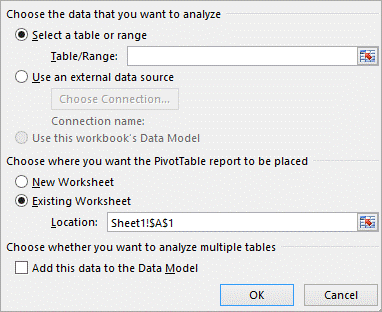
3. Choose the data that you want to analyze>Select a table or range.

4. Verify the cell range in Table/Range.
5. Select New worksheet under Choose where you want the PivotTable report to be placed. This will place the PivotTable in a new worksheet. Or you can change it to Existing worksheet, thereafter, selecting the location you want the PivotTable to appear.
6. Click OK.
VLookup
If you need to find things in a table or a range by row, use VLOOKUP. For example, finding an employee name based on employee ID. The VLOOKUP function works like:
=VLOOKUP(What, where you want to look up, the column number in the range containing the value to return, return an Approximate or Exact match).
Filters
Use filters to pay attention to the data you want to see while simultaneously hiding some of the data in a table temporarily. Steps to Filter data:
1. Select any cell within the range.
2. Choose Data > Filter.

3. Click the column header arrow.
4. Select Text Filters or Number Filters, then select a comparison, like Between.

5. Enter the filter criteria and click OK.


